Basic Statistics in DMAIC

Facebook
Twitter
LinkedIn
Email
You are here:

By now probably have realised Lean Six Sigma is an effective methodology for increasing organizational efficiency and quality. To achieve this Lean Six Sigma is fundamentally based on statistical techniques to identify areas for improvement and track progress.

Therefore it is important to gain an understanding of fundamental statistical concepts such as mean, median, and mode, standard deviation, range, central tendency, and percentiles is critical for anyone interested in implementing Lean Six Sigma in their organisation.

Table of Contents

Basic Statistical Concepts

The Importance of understanding key statisical concepts in Lean Six Sigma

Statistical ideas are critical in finding areas for improvement and assessing progress in Lean Six Sigma. Understanding basic statistical principles enables practitioners of Lean Six Sigma to evaluate data, discover patterns and trends, and make data-driven decisions.

For example, the concept of central tendency, which encompasses metrics such as mean, median, and mode, can be used to comprehend a process’s or system’s normal performance. This data can then be utilised to spot outliers and regions where performance deviates from the norm.

Similarly, standard deviation is used to determine the spread of data and the amount of variation in a process or system. This data can be used to define performance goals and track progress toward those goals.

Understanding fundamental statistical concepts such as mean, median, mode, standard deviation, range, central tendency, and percentiles is critical for everyone interested in implementing Lean Six Sigma in their business. These principles provide useful insights into process and system performance, helping organisations to detect patterns, trends, and outliers that may be leveraged to drive improvement.

What are the basic staticial concepts in Lean Six Sigma?

There are a range of basic statistical concepts you need to gain an understanding of at the Lean Six Sigma Yellow belt level to support understanding and exploring of data in Lean Six Sigma project which includes:

Mean, Median, and Mode: These are central tendency metrics that describe the average value of a data set. The arithmetic average is the mean, the median is the midway number, and the mode is the most commonly occurring value.

Standard Deviation: This is a measure of the spread of data, and it tells us how much variation there is in a data set.

Range: This is a measure of the spread of data and tells us the difference between the lowest and highest values in a data set.

Central Tendency: This relates to a data set’s central value, which can be stated using mean, median, or mode.

Percentiles: Percentiles divide a data set into 100 equal parts, and tell us what percentage of the data falls below a certain value.


Furthermore, additional statistical concepts include Pareto charts and Scatter Plots which we have covered previously. Then there are Control charts which we will cover in the control stage of DMAIC.


Mean, Median and Mode and Central Tendency

What is Central Tendency?

The central tendency of a data collection refers to its average or usual value. It is a measure of where the data’s middle or centre is located. The mean, median, and mode are the most widely used measures of central tendency.

Mean: The mean is the arithmetic average of a data set. It is calculated by adding all of the values in the data set and then dividing the total number of values by the number of values. The mean is a measure of the data set’s centre, but it can be influenced by extreme numbers or outliers.

Median: The median is the middle value of a data set when it is arranged in numerical order. Half of the values in the data set are higher than the median, while the other half are lower. Extreme values or outliers have no effect on the median.

Mode: The mode is the most frequently occurring value in a data set. A data set can have a single mode, several modes, or no mode at all.

Central tendency is often used in statistics to describe the typical value of a data set and to identify patterns, trends, and outliers. It can also be used to compare data sets and draw conclusions about the population from which the data was drawn.

Basic statistics in DMAIC

It is crucial to highlight that the best measure of central tendency depends on the data set; sometimes the mean is the best measure, sometimes the median, and sometimes the mode. It is critical to analyse the data distribution, whether it is symmetric or skewed, and whether it contains outliers. sampled.

Choosing the appropriate measure of central tendency is dependent on the data collection and the type of research being performed. Here are some tips to help you decide which measure of central tendency is best for your data set:

Symmetric distributions: If your data collection is symmetric and free of outliers, the mean, median, and mode will all be the same (middle example above). Any of the three measures can be employed in this scenario.

Skewed distributions: The mean, median, and mode of your data collection will be different if it is skewed (left and right examples above). Because it is unaffected by extreme values or outliers, the median is the best measure of central tendency in this circumstance.

Outliers: If your data collection contains outliers, the mean will be impacted and may not be reflective of the data set’s typical value. Because it is unaffected by outliers, the median is a better estimate of central tendency in this scenario.

Nominal Data: No mean or median can be calculated with nominal data, but mode can be used to understand the most frequent number.

Data with many peaks: If the data includes multiple peaks, it is multimodal, and mode can be utilised to comprehend the various sorts of usual values in the data set.

It is critical to remember that while evaluating data, it is always necessary to look at the data graphically, such as using a histogram or boxplot, to obtain a feel of the distribution and outliers. This allows you to make a more educated judgement about which measure of central tendency is best for your data collection.


How is this used in Lean Six Sigma?

To provide a more full view of a process or system’s performance, central tendency is frequently used in conjunction with other statistical concepts such as standard deviation, range, and control charts in Lean Six Sigma.

For instance, if a process has a mean of 6 minutes and a standard deviation of 1 minute, this data can be utilised to create a performance objective of 6 minutes +/-1 minute. When a process performs at the median, it signifies that half of the data points are above the median and half are below it. If you have not learnt standard deviation before, dont worry we will explain it clearly below.

Furthermore, central tendency measures can be used to discover patterns and trends in data sets, such as when a process produces more faults than usual or when customer complaints increase. These patterns and trends can then be utilised to identify problem areas and track improvements over time.

Standard Deviation

What is Standard Deviation?

The standard deviation is a measure of data spread that shows us how much variety exists in a data set. It is a statistical concept that indicates how far individual data points in a set depart from the mean of the set.

It is calculated by calculating the difference between each data point and the mean, squaring those differences, and then averaging the squared differences. Finally, the standard deviation is calculated by taking the square root of this average.

A low standard deviation implies that the majority of the data points in a set are close to the mean, whereas a high standard deviation suggests that the data points are more spread out and deviate from the mean more widely.

In statistics, standard deviation can be used in a variety of ways, including:

To understand how much variation there is in a data set: The standard deviation is a numerical measurement that quantifies the degree of variation in a data set. Knowing a process’s standard deviation helps you to construct a range of expected values, such as the process mean plus or minus 3 times the standard deviation.

To set performance targets and measure progress towards those targets: Standard deviation can also be used to determine the degree of variation in a process and to establish performance goals. A customer care procedure with a standard deviation of 30 seconds, for example, can set a target of keeping calls under 90 seconds (mean+3*standard deviation) to have a high level of confidence that most calls will be under that time.

To identify and compare the variability of different data sets: To compare the variability of different data sets, standard deviation can be employed. A lower standard deviation process is thought to be more consistent and predictable than a larger standard deviation process.

To detect outliers or extreme values in a data set: A standard deviation can be used to identify outliers or extreme values in a data set. Outliers are values that go outside of the predicted range (mean plus or minus 3 times the standard deviation). Outliers can be studied to see whether they are genuine data points or errors.

In summary, standard deviation is a great tool for understanding how much variety exists in a data collection, setting performance targets, and tracking progress.

The Bell Curve

The bell curve, also known as the normal distribution or Gaussian distribution, is a probability distribution that describes the distribution of a continuous variable. It is a symmetric distribution, with the majority of observations clustering around the mean value, and fewer observations as we move farther away from the mean. The shape of the bell curve is determined by the mean and standard deviation of the data. The mean represents the centre of the distribution, and the standard deviation represents how spread out the data is from the mean. A larger standard deviation results in a flatter curve, while a smaller standard deviation results in a taller, narrower curve.
 
The normal distribution has several important properties:
 
  • Because the area under the curve equals one, the total probability of all conceivable outcomes is one.
  • The mean, median, and mode are all the same.
  • Asymptotically, the curve approaches but never reaches the x-axis.
  • µ is the greek letter for “mu” and is used to denote the mean
  • σ is the symbol for sigma or standard deviations
  • In a normal distribution Bell curve
    • 99.72% of data points fall between -3 standard deviations and +3 standard deviations from the mean
    • 95.44% of data points fall between +2 standard deviation and -2 standard deviations from the mean
    • 68.28% of data points fall between +1 standard deviation and -1 standard deviation from the mean.
Standard deviation bell curve

The normal distribution is widely used in statistics and probability because it can approximate many real-world phenomena, such as the distribution of human heights and weights, and the distribution of errors in measurements. It is also often used as a reference distribution to compare other distributions against. 

In SPC, the normal distribution is used to understand and analyse process data, to check if it follows a normal distribution or not.

In SPC, standard deviation is used to calculate control limits for control charts and also used in process capability analysis. Understanding the standard deviation and the range of +1 and -1 standard deviation from the mean is important in order to interpret the results of control charts and make informed decisions on how to improve a process.

If we rotate the bell curve 90 degres clockwise and add a line graph onto it, you can see the normal distribution of data points. Example image below. However, we will cover control charts later in the course, but this is to help you visualise the standard deviation of data points and control charts.

  • The UCL is the Upper Control Limit and is always + 3 standard deviations from the mean
  • The LCL is the Lower Control Limit and is always – 3 standard deviations from the mean.
  • All data points within the UCL and LCL is classed as common cause variation as it is statistically likely and accounts for 99.72% of all data points.
  • Any data points outside the UCL and LCL is classed as special cause variation as it is statistically unlikely and will only occur around 2.8 times in 1000 data points. This is so rare that any data points that fall outside the control limits should be explored to understand why it happened. 
  • The data itself is what sets the control limits so if the input data changes so too will the control limits.
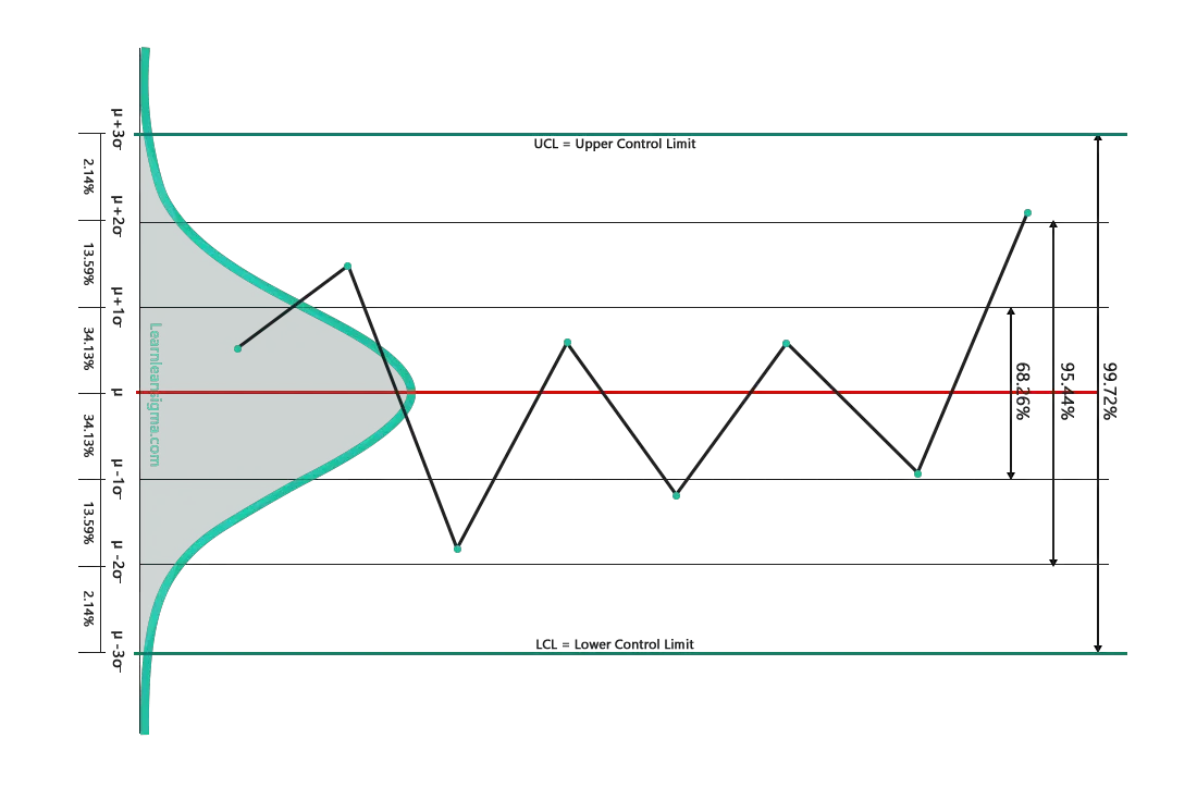
Bell Curve Standard Deviation Control Chart

When we refer to +1 or -1 standard deviations from the mean, we are referring to a range of values that are either 1 standard deviation above or 1 standard deviation below the mean. For example, if the mean of a set of data is 50 and the standard deviation is 5, then +1 standard deviation from the mean would be 55 and -1 standard deviation from the mean would be 45. Therefore 68.26% of all data points will fall between 55 and 45.

The spread of data

In statistics, standard deviation is a measure of a data set’s spread. It indicates how far the data in a set deviates from the mean. The standard deviation is computed by squaring the difference between each data point and the mean, adding the sum, and then taking the square root of that amount.

Standard deviation is used in the context of Statistical Process Control (SPC) to find trends in a data collection and assess if the variation in the data is due to a common cause or a special reason.

Common cause variation is the inherent variation that is always present in a process and is a result of the natural variation of the process. It is also known as random variation and is caused by factors that are hard to control or measure, such as measurement error. Common cause variation is usually stable and predictable and follows a normal distribution.

Special cause variation, on the other hand, is caused by specific factors that are not inherent in the process. It is also known as assignable variation and is caused by factors that can be controlled or measured, such as changes in equipment or staff. Special cause variation is usually unstable and unpredictable and does not follow a normal distribution.

If the data has a normal distribution and the standard deviation is within the permitted range, it is deemed common cause variation and no further action is required in SPC. However, if the data does not follow a normal distribution and the standard deviation is outside the permitted range, it is deemed special cause variation and requires further research to determine the cause and make appropriate process improvements.

In summary, standard deviation is a measure of a data set’s spread, and it is used in SPC to find patterns in a data set and assess if the variation in the data is due to a common or special source. Understanding the distinction between common and special cause variation is critical for identifying the source of variability and making appropriate process modifications.


How to calculate Standard Deviation?

The standard deviation is a measure of the spread of a set of data. It is a measure of how far a set of numbers is spread out from its mean. To calculate the standard deviation, you need to follow these steps:

  • Calculate the mean of the data set. This is done by adding all the values in the data set and then dividing by the number of values.
  • Subtract the mean from each data point to find the deviation of each point from the mean.
  • Square each deviation and find their sum.
  • Divide the sum of the squared deviations by the number of data points (n) minus 1. This gives you the variance.
  • Take the square root of the variance to find the standard deviation.

For example, let’s say we have a data set of 5 values: 2, 4, 5, 8, 9.

Example with data:

Step 1: Find the Mean (2+4+5+8+9=28) 28/5 = 5.6

calculate the mean

Step 2: Calculate the deviation of each point from the mean. e.g. (2-5.6 = -3.6)

deviation from mean

Step 3: Square each deviation. Squaring a number is multiplying it by itself e.g. -3.6 x -3.6 = 12.96. 

Note: Negative numbers become positive numbers

squared deviation
Step 4: Add the squared deviations together (12.96 + 2.56 + 0.36 + 5.76 + 11.56 = 33.20) divide by the number of data points. 5 = 33.2/5 = 6.64
Step for standard deviation calculation
Step 5: Find the square root of 6.64. On a calculator type in 6.64 then press  √ = 2.57
 

Therefore, the standard deviation of 2, 4, 5, 8 and 9 = 2.57

Although you can use standard deviation calculators link the one below, it is useful to understand how to calculate standard deviations as you may need to calculate it for a large data set of 1000 + Numbers


Standard Deviation Calculator


How is standard deviation applied to Lean Six Sigma Projects?

Standard deviation is used in Lean Six Sigma projects to:

Measure process performance: Standard deviation is used to measure the spread of a data set and to determine whether a process is in control or out of control. The process is regarded to be under control if the standard deviation is within acceptable norms. If the standard deviation is outside of the acceptable limits, the process is considered to be out of control and further investigation is needed.

Identify special cause variation: In a process, standard deviation is also utilised to identify special cause variation. Special cause variation is caused by external influences that cannot be controlled or measured in the process. Identifying unique cause variation is critical for making appropriate process adjustments and enhancing process performance.

Set control limits: In Lean Six Sigma, control limits are set depending on the data’s standard deviation. Control limits are used to determine whether or not a process is under control. The process is regarded to be in control if the data falls within the control limits. If the data exceeds the control limitations, the process is said to be out of control and needs further investigation

Determine process capability: The standard deviation is also used to determine a process’s capabilities. Process capability is a measurement of how well a process can produce results within a given range. By comparing the standard deviation of the process to the tolerance range, you may establish how well the process meets client requirements and discover opportunities for improvement.

Set process improvement targets: Standard deviation is used to set process improvement targets. Understanding a process’s existing standard deviation allows you to set realistic targets for improvement. For example, if a process has a standard deviation of 2, you can establish a goal of reducing it to 1.5 or 1.


Range

What is Range?

In statistics, the range is a measure of a data set’s spread. It is calculated by subtracting the greatest and lowest values in a data collection. The range indicates the dispersion of the data and is a simple measure of variability. It is defined as the distance between a data set’s largest and smallest observations.

For example, if a data collection has the numbers 2, 4, 5, 8, 9, the range is 9 (the greatest value) – 2 (the smallest value) = 7. This signifies that the data spans a range of 7 units, which might help you determine how dispersed the data is.

The range is a simple measure of variability that can be used to quickly identify outliers; however, it is sensitive to the presence of outliers and does not account for data distribution. Other measures of variability, such as variance and standard deviation, are more resilient and provide a more accurate portrayal of data spread, particularly when the data is not evenly distributed.

In summary, range is a simple measure of a data set’s spread that is determined by subtracting the greatest and smallest values from the data set. It is a rapid technique to analyse data variability, but it is susceptible to outliers and does not take into consideration the distribution of the data.


How is Range used in Lean Six Sigma?

In Lean Six Sigma, the range is used in the following ways:

Measure process performance: The range is used to identify whether a process is in control or out of control by measuring the spread of a data set. Calculating the range allows you to quickly determine whether the process is delivering results within an acceptable range or if there are outliers.

Identify special cause variation: In a process, the range is also utilised to identify special cause variation. Special cause variation is caused by external influences that cannot be controlled or measured in the process. You may find special cause variance in the process and make necessary adjustments to improve performance by detecting outliers in the data.

Set control limits: In Lean Six Sigma, control limits are set depending on the data range. Control limits are used to determine whether or not a process is under control. The process is regarded to be in control if the data falls within the control limits. If the data exceeds the control limitations, the process is deemed out of control, and additional examination is required.

Determine process capability: Range can be used as a measure of process capability, to determine how well a process is capable of producing results within a specific range. By comparing the process’s range to the tolerance range, you can determine how well the process is able to meet customer requirements and identify areas for improvement.


Percentiles

What are Percentiles?

Percentiles are used in statistics to divide a data collection into 100 equal portions. Percentiles are used to define a value’s position within a data set. Each percentile denotes a value below which a specific percentage of observations in a data set fall.

The 50th percentile, often known as the median, is the value that divides the lowest 50% of data from the highest 50% of data, for example. When a data collection is sorted in ascending order, the median value is the midway value.

The 25th percentile, commonly known as the first quartile, divides the data into the bottom 25% and the top 75%. The first quartile is defined as the value at which 25% of the observations fall. Similarly, the 75th percentile, often known as the third quartile, divides the data into the lowest 75% and the highest 25%. The number in the third quartile is below which 75% of the observations fall.

Because the median and quartiles are unaffected by outliers, percentiles are useful for analysing the distribution of a data collection. Percentiles are also used to calculate and compare various measures of central tendency and variability, such as interquartile range (IQR), which is the difference between the first and third quartiles and is used to detect outliers and skewness in data.

To summarise, percentiles divide a data set into 100 equal pieces. Percentiles represent a value’s position within a data set. Percentiles can be used to comprehend a data set’s distribution, compare alternative measures of central tendency and variability, and discover outliers and skewness in data.


How are Percentiles used in Lean Six Sigma?

Percentiles are used in Lean Six Sigma to analyse the distribution of a data collection and detect patterns in the process. Percentiles are important for determining a value’s relative position within a data collection and comparing different metrics of central tendency and variability.

Here are some examples of how percentiles are utilised in Lean Six Sigma:

Detect patterns: Percentiles are used to comprehend a data set’s distribution and to identify patterns. Calculating the percentiles of a data collection allows you to easily determine the median, quartiles, and other percentiles, which can help you comprehend the data distribution and identify patterns.

Determine process capability: Percentiles are used to determine a process’s process capability. Process capability is a measurement of how well a process can produce results within a given range. You can determine how well the process meets client expectations and discover opportunities for improvement by comparing its percentiles to the tolerance range.

Determine special cause variation in a process: Percentiles can also be used to determine special cause variation in a process. You may find special cause variance in the process and make necessary adjustments to improve performance by detecting outliers in the data.

Establish control limits: Control limits in Lean Six Sigma are established based on data percentiles. Control limits are used to determine whether or not a process is under control. The process is regarded to be in control if the data falls within the control limits. If the data exceeds the control limitations, the process is deemed out of control, and additional examination is required.

In summary, in Lean Six Sigma, percentiles are used to understand the distribution of a data set and detect patterns in the process. They can be used to determine process capability, identify special cause variation, and set control limits. You may obtain a deeper understanding of a process and find opportunities for improvement by using percentiles, which is critical to attaining success in Lean Six Sigma projects.


Conclusion

To summarise, important statistical principles are critical in Lean Six Sigma because they enable practitioners to examine data, uncover patterns and trends, and make data-driven decisions. Concepts such as central tendency, which encompasses mean, median, and mode, can be used to understand the usual behaviour of a process or system and identify outliers. The standard deviation of a process or system is used to determine the spread of data and the amount of variation.

Range and percentiles are further metrics of data distribution. In addition, other statistical concepts utilised in Lean Six Sigma to assess and optimise processes include Pareto charts, Scatter Plots, and Control charts. It is vital to note that the appropriate measure of central tendency and other statistical notions are determined by the data distribution and any outliers in the data set.


What's Next?

We have now covered all the necessary statistics and analysis of a Lean Six Sigma Yellow Belt. Next we will cover at the Improve phase of DMAIC and start by covering eliminating waste and work balancing.